Preface: The following article was co-written with Shashank Kapadia and was first published on Towards Data Science on July 4, 2023.

This article presents a summary of information about the given topic. It should not be considered original research. The information and code included in this article have may be influenced by things I have read or seen in the past from various online articles, research papers, books, and open-source code.

Introduction
Theoretical Framework
Data Overview
Starting Point: The Baseline Model
Fine-Tuning the Model
Evaluating the Results
Closing Thoughts

Introduction

In today’s world, the availability of pre-trained NLP models has greatly simplified the interpretation of textual data using deep learning techniques. However, while these models excel in general tasks, they often lack adaptability to specific domains. This comprehensive guide aims to walk you through the process of fine-tuning pre-trained NLP models to achieve improved performance in a particular domain.

Motivation

Although pre-trained NLP models like BERT and the Universal Sentence Encoder (USE) are effective in capturing linguistic intricacies, their performance in domain-specific applications can be limited due to the diverse range of datasets they are trained on. This limitation becomes evident when analyzing relationships within a specific domain.

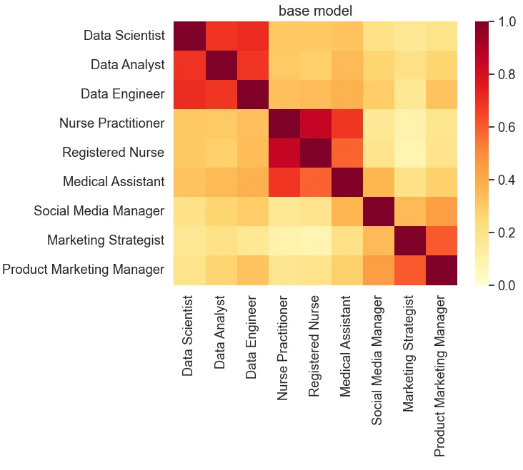
For example, when working with employment data, we expect the model to recognize the closer proximity between the roles of ‘Data Scientist’ and ‘Machine Learning Engineer’, or the stronger association between ‘Python’ and ‘TensorFlow’. Unfortunately, general-purpose models often miss these nuanced relationships.

The table below demonstrates the discrepancies in the similarity obtained from a base multilingual USE model:

alt text

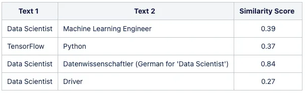
To address this issue, we can fine-tune pre-trained models with high-quality, domain-specific datasets. This adaptation process significantly enhances the model’s performance and precision, fully unlocking the potential of the NLP model.

When dealing with large pre-trained NLP models, it is advisable to initially deploy the base model and consider fine-tuning only if its performance falls short for the specific problem at hand.

This tutorial focuses on fine-tuning the Universal Sentence Encoder (USE) model using easily accessible open-source data.

Theoretical Overview

Fine-tuning an ML model can be achieved through various strategies, such as supervised learning and reinforcement learning. In this tutorial, we will concentrate on a one(few)-shot learning approach combined with a siamese architecture for the fine-tuning process.

Methodology

In this tutorial, we utilize a siamese neural network, which is a specific type of Artificial Neural Network. This network leverages shared weights while simultaneously processing two distinct input vectors to compute comparable output vectors. Inspired by one-shot learning, this approach has proven to be particularly effective in capturing semantic similarity, although it may require longer training times and lack probabilistic output.

A Siamese Neural Network creates an ‘embedding space’ where related concepts are positioned closely, enabling the model to better discern semantic relations.

alt text

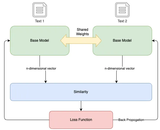
Twin Branches and Shared Weights: The architecture consists of two identical branches, each containing an embedding layer with shared weights. These dual branches handle two inputs simultaneously, either similar or dissimilar.
Similarity and Transformation: The inputs are transformed into vector embeddings using the pre-trained NLP model. The architecture then calculates the similarity between the vectors. The similarity score, ranging between -1 and 1, quantifies the angular distance between the two vectors, serving as a metric for their semantic similarity.
Contrastive Loss and Learning: The model’s learning is guided by the “Contrastive Loss,” which is the difference between the expected output (similarity score from the training data) and the computed similarity. This loss guides the adjustment of the model’s weights to minimize the loss and enhance the quality of the learned embeddings.

To learn more about one(few)-shot learning, siamese architecture, and contrastive loss, refer to the following resources:

The complete code is available as a Jupyter Notebook on GitHub

Data Overview

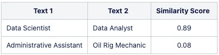
For the fine-tuning of pre-trained NLP models using this method, the training data should consist of pairs of text strings accompanied by similarity scores between them.

The training data follows the format shown below:

alt text

In this tutorial, we use a dataset sourced from the ESCO classification dataset, which has been transformed to generate similarity scores based on the relationships between different data elements.

Preparing the training data is a crucial step in the fine-tuning process. It is assumed that you have access to the required data and a method to transform it into the specified format. Since the focus of this article is to demonstrate the fine-tuning process, we will omit the details of how the data was generated using the ESCO dataset.

The ESCO dataset is available for developers to freely utilize as a foundation for various applications that offer services like autocomplete, suggestion systems, job search algorithms, and job matching algorithms. The dataset used in this tutorial has been transformed and provided as a sample, allowing unrestricted usage for any purpose.

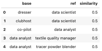
Let’s start by examining the training data:

import pandas as pd

# Read the CSV file into a pandas DataFrame
data = pd.read_csv("./data/training_data.csv")

# Print head
data.head()

alt text

Starting Point: The Baseline Model

To begin, we establish the multilingual universal sentence encoder as our baseline model. It is essential to set this baseline before proceeding with the fine-tuning process.

For this tutorial, we will use the STS benchmark and a sample similarity visualization as metrics to evaluate the changes and improvements achieved through the fine-tuning process.

The STS Benchmark dataset consists of English sentence pairs, each associated with a similarity score. During the model training process, we evaluate the model’s performance on this benchmark set. The persisted scores for each training run are the Pearson correlation between the predicted similarity scores and the actual similarity scores in the dataset.

These scores ensure that as the model is fine-tuned with our context-specific training data, it maintains some level of generalizability.

# Loads the Universal Sentence Encoder Multilingual module from TensorFlow Hub.
base_model_url = "https://tfhub.dev/google/universal-sentence-encoder-multilingual/3"
base_model = tf.keras.Sequential([
    hub.KerasLayer(base_model_url,
                   input_shape=[],
                   dtype=tf.string,
                   trainable=False)
])

# Defines a list of test sentences. These sentences represent various job titles.
test_text = ['Data Scientist', 'Data Analyst', 'Data Engineer',
             'Nurse Practitioner', 'Registered Nurse', 'Medical Assistant',
             'Social Media Manager', 'Marketing Strategist', 'Product Marketing Manager']

# Creates embeddings for the sentences in the test_text list. 
# The np.array() function is used to convert the result into a numpy array.
# The .tolist() function is used to convert the numpy array into a list, which might be easier to work with.
vectors = np.array(base_model.predict(test_text)).tolist()

# Calls the plot_similarity function to create a similarity plot.
plot_similarity(test_text, vectors, 90, "base model")

# Computes STS benchmark score for the base model
pearsonr = sts_benchmark(base_model)
print("STS Benachmark: " + str(pearsonr))

alt text

STS Benchmark (dev): 0.8325

Fine Tuning the Model

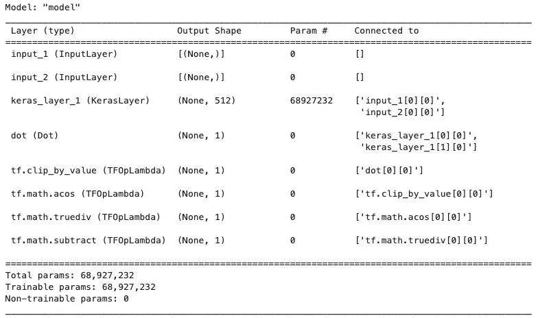
The next step involves constructing the siamese model architecture using the baseline model and fine-tuning it with our domain-specific data.

# Load the pre-trained word embedding model
embedding_layer = hub.load(base_model_url)

# Create a Keras layer from the loaded embedding model
shared_embedding_layer = hub.KerasLayer(embedding_layer, trainable=True)

# Define the inputs to the model
left_input = keras.Input(shape=(), dtype=tf.string)
right_input = keras.Input(shape=(), dtype=tf.string)

# Pass the inputs through the shared embedding layer
embedding_left_output = shared_embedding_layer(left_input)
embedding_right_output = shared_embedding_layer(right_input)

# Compute the cosine similarity between the embedding vectors
cosine_similarity = tf.keras.layers.Dot(axes=-1, normalize=True)(
    [embedding_left_output, embedding_right_output]
)

# Convert the cosine similarity to angular distance
pi = tf.constant(math.pi, dtype=tf.float32)
clip_cosine_similarities = tf.clip_by_value(
    cosine_similarity, -0.99999, 0.99999
)
acos_distance = 1.0 - (tf.acos(clip_cosine_similarities) / pi)

# Package the model
encoder = tf.keras.Model([left_input, right_input], acos_distance)

# Compile the model
encoder.compile(
    optimizer=tf.keras.optimizers.Adam(
        learning_rate=0.00001,
        beta_1=0.9,
        beta_2=0.9999,
        epsilon=0.0000001,
        amsgrad=False,
        clipnorm=1.0,
        name="Adam",
    ),
    loss=tf.keras.losses.MeanSquaredError(
        reduction=keras.losses.Reduction.AUTO, name="mean_squared_error"
    ),
    metrics=[
        tf.keras.metrics.MeanAbsoluteError(),
        tf.keras.metrics.MeanAbsolutePercentageError(),
    ],
)

# Print the model summary
encoder.summary()

alt text

Fit the model

# Define early stopping callback
early_stop = keras.callbacks.EarlyStopping(
    monitor="loss", patience=3, min_delta=0.001
)

# Define TensorBoard callback
logdir = os.path.join(".", "logs/fit/" + datetime.now().strftime("%Y%m%d-%H%M%S"))
tensorboard_callback = keras.callbacks.TensorBoard(log_dir=logdir)

# Model Input
left_inputs, right_inputs, similarity = process_model_input(data)

# Train the encoder model
history = encoder.fit(
    [left_inputs, right_inputs],
    similarity,
    batch_size=8,
    epochs=20,
    validation_split=0.2,
    callbacks=[early_stop, tensorboard_callback],
)

# Define model input
inputs = keras.Input(shape=[], dtype=tf.string)

# Pass the input through the embedding layer
embedding = hub.KerasLayer(embedding_layer)(inputs)

# Create the tuned model
tuned_model = keras.Model(inputs=inputs, outputs=embedding)

Evaluation

Now that we have the fine-tuned model, let’s re-evaluate it and compare the results to those of the base model.

# Creates embeddings for the sentences in the test_text list. 
# The np.array() function is used to convert the result into a numpy array.
# The .tolist() function is used to convert the numpy array into a list, which might be easier to work with.
vectors = np.array(tuned_model.predict(test_text)).tolist()

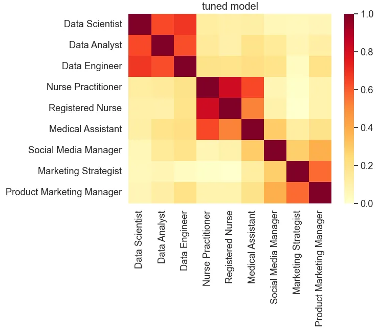
# Calls the plot_similarity function to create a similarity plot.
plot_similarity(test_text, vectors, 90, "tuned model")

# Computes STS benchmark score for the tuned model
pearsonr = sts_benchmark(tuned_model)
print("STS Benachmark: " + str(pearsonr))

alt text

STS Benchmark (dev): 0.8349

Based on fine-tuning the model on the relatively small dataset, the STS benchmark score is comparable to that of the baseline model, indicating that the tuned model still exhibits generalizability. However, the similarity visualization demonstrates strengthened similarity scores between similar titles and a reduction in scores for dissimilar ones.

Closing Thoughts

Fine-tuning pre-trained NLP models for domain adaptation is a powerful technique to improve their performance and precision in specific contexts. By utilizing quality, domain-specific datasets and leveraging siamese neural networks, we can enhance the model’s ability to capture semantic similarity.

This tutorial provided a step-by-step guide to the fine-tuning process, using the Universal Sentence Encoder (USE) model as an example. We explored the theoretical framework, data preparation, baseline model evaluation, and the actual fine-tuning process. The results demonstrated the effectiveness of fine-tuning in strengthening similarity scores within a domain.

By following this approach and adapting it to your specific domain, you can unlock the full potential of pre-trained NLP models and achieve better results in your natural language processing tasks

Domain Adaptation: Fine-Tune Pre-Trained NLP Models

A step-by-step guide to fine-tuning pre-trained NLP models for any domain

Table of Contents

Introduction

Motivation

Theoretical Overview

Methodology

Data Overview

Starting Point: The Baseline Model

Fine Tuning the Model

Fit the model

Evaluation

Closing Thoughts