Demo

Intro

As a part of the SharpestMinds mentorship program, mentees are encouraged to build a full-stack machine learning project with oversight from their mentor. My mentor, Brian Godsey, and I started this project phase out by kicking around different ideas and exploring potential data sources. I had just moved to a new neighborhood in Boston where street parking was much more difficult to find, and I was interested to see if I could build some type of forecasting tool that would help me find parking faster. It was this idea that became the basis for the project. I will use this post to try to summarize the project in the following steps:

1. Data acquisition, storage, and exploratory analysis
2. Model building and testing
3. Building the web app and the associated software engineering tasks

Data

Data Acquisition and Storage

I began my search for parking related data in the City of Boston open data hub hoping that I could start with a data set that could alleviate some of my own parking problems. Unfortunately, I couldn’t find a robust enough data set to make predictions with. I started searching for parking related data sets in other public data portals and eventually found that the City of Melbourne had installed in-ground sensors to many of their parking spaces in the center of the city and had been recording the data from these sensors. These sensors allow city officials to better understand how parking is being utilized as a resource in the city. The city also publishes all the historical data onto the web so that the public can have access to it. This data set would prove to be robust enough to perform some predictive modeling with and be the data set that this project would be built upon.

The City of Melbourne has parking sensor data going back to 2011 and the data for each year is stored in a single file. Each year of data has between 20 M and 50 M observations and each year can occupy almost 8 GB on disk. This isn’t necessarily “big data”, but it’s big enough that I couldn’t load it into memory on my machine. I chose to put the data into a MongoDB database because of its easy setup. After installing MongoDB and the Python driver, PyMongo; I was able to connect to the database, create an initial collection (the Mongo equivalent of a table), and write a for-loop to read and insert the data in chunks. In a happy coincidence I later learned that MongoDB also supports GeoJSON, which is a format for encoding geographical data. Along with the parking event data, the City of Melbourne also provides a data set that has all the geographic information of the parking spots in this GeoJSON format. This data includes lat/long coordinates that define the geometry of each parking space as well as an identifier to map each spot back to the parking event data. This would be useful later for finding nearby parking spots as well as accurately plotting their position on a map.

Exploratory Analysis

Now that I had the data stored in a database, I could start exploring the data and looking for patterns. I started with getting some initial counts of total events and events in different city areas which were included in the data. I then started looking more specifically the observations and the timestamps associated with them. Each observation in the data is a segment of time with an arrival time, a departure time, and an indicator of whether the space is occupied or unoccupied. At first, I had assumed that each observation would be a time segment where the space was occupied, but I soon noticed that within a single space there were duplicate timestamps. This is because the times when the space is empty are also logged as observations but with an indicator variable showing that the space is unoccupied. What this looks like in the real world is that when a car occupies a space, an event is logged with an arrival time and an indicator that the space is occupied. When the car leaves the space, the initial event is logged with a departure time and a new event begins. The departure time associated with the car leaving the space becomes the arrival time for this second event and the occupancy indicator is set to unoccupied. When another car arrives in the space, that time is logged as the departure time of the previous unoccupied event. Understanding how these events were logged would become important later as I needed to start quantifying the occupancy rates of different spaces.

One of the first things I did was to visualize the distribution of event times throughout the day. The following chart shows the frequency of arrival times for each hour of the day, or how many times during each hour someone pulled into a parking space and started a parking event:

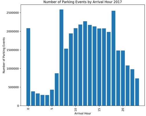
This chart shows the parking activity for each hour of the day, and appears to have a pattern you might expect. Most of the parking events happen throughout the middle of the day and activity tapers off overnight. This means that when we want to start making predictions that the hour of the day will be an important feature.

The spikes at midnight, 7 AM, and 6 PM stand out and are an artifact of the sensor behavior. Each sensor resets at midnight, so every sensor starts a new observation at that point which shows up as a new event with an arrival time of midnight. There are also many meters where parking is only allowed from 7:30 AM until 6:30 PM, and these meters automatically start a new event at those times.

The next thing I wanted to look into was to see if there was a difference in the number of parking events for each day type. I made a similar hourly histogram as above, but created one for each day of the month to see if I could see a difference in parking events by day. The following chart shows this visualization for the month of June:

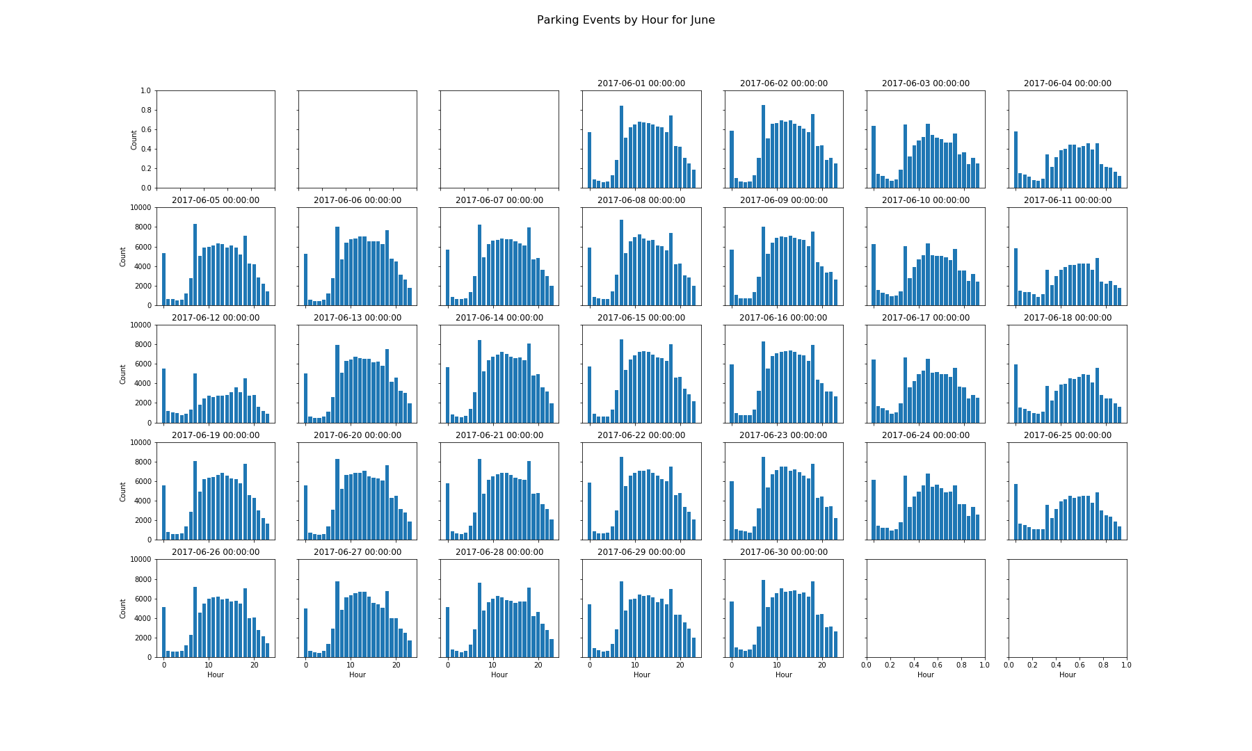
This chart is set up similar to a calendar, although it is arranged from left to right as Monday - Sunday. You can see that the weekdays exhibit a similar pattern, Saturdays seem to have a slightly lower amount of events, and Sundays even lower still. June 12th also appears to have fewer events than the other Mondays. This particular Monday is the Queen’s Birthday and is a national holiday in Australia. After looking at this chart I knew that the day-type would also be an important feature to consider when predicting parking.

Modeling

Query-Based Model

Because I eventually want to be able to point a user in the direction of open parking spaces, I need a way to model this behavior to make predictions. The first method I tried was a query-based approach which is essentially using frequentist inference to make a prediction on availability of a spot. Provided a space, a date, and a time of interest; we’ll query for previous parking events that occur on the same day-type and around the same time. This query was built using the following steps:

1. Create a list of dates prior to the date of interest with each date 7 days apart to match day-type
2. For each date, query for events where:
   a. The space identifier matches the space of interest
   b. The arrival time of the event happens within a predefined time window around the time of interest
   c. The departure time of the event happens within a predefined time window around the time of interest

For instance, if you want to know if you can park in a spot at 3:30 PM on a Friday afternoon, the query will find all the parking events that happened in the past 10 Fridays between 3:00 and 4:00 PM, and then calculate the percentage of time that the spot was open. This percentage of available time becomes the prediction of that space being available.

For the final user-facing application, I knew that I wanted to display predictions at a block level rather than an individual space level. To do this, I followed a very similar process to the original spot level modeling, but instead of looking at the percent of time that a spot was open, I looked at the percent of time that at least a single spot in the block was open.

Tuning the Model

The query described above has two tunable parameters:

1. the number of previous days to include
2. the size of the time window

To tune these, I created a training set of randomly generated dates and times and queried each space to see if it was occupied or unoccupied at those times. I then used the query from above to make predictions and evaluated the predictions using a Log-Loss score.

A Log-Loss score is commonly used to score the performance of binary classification models where the two inputs are the actual labels and the model’s probability values between 0 and 1. The Log-Loss score of a perfect model is 0, and the score will increase for predictions that are increasingly wrong. For instance a prediction of 0.1 for an observation with a value of 1 will have a higher Log-Loss than a prediction of 0.7 for the same observation of 1. A prediction of 1 for an observation of 1 would have a Log-Loss of 0. This metric would help to tune my query parameters as it captures more nuance of the predictions than other metrics like accuracy.

I performed a grid search over the two parameters to minimize the Log-Loss error metric. This query-based method has an inherent trade off between capturing enough previous observations and ensuring that those observations are representative of the target time being predicted for. If the query doesn’t capture enough previous events, it won’t have a large enough sample size to be able to make an accurate prediction and may be influenced by noise in the data. If the query captures too many events, it may capture parking behaviors that are not representative of the time and date of interest. This trade-off is evident in the results of the grid search over these parameters: as each parameter increased, the scores began to drop towards a minimum. The scores then began to increase as the time window became too large. The following table shows Log-Loss scores across several values of the query parameters:

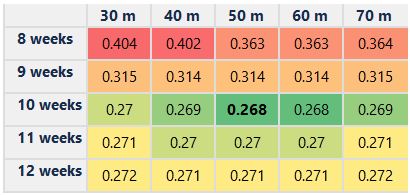
You can see in the table that using 10 previous weeks and a time window of 50 minutes provided the lowest Log-Loss score against the training set. With these parameters set, I created a test set of data with another set of randomly generated dates and times to measure the performance.

Model Performance and Prediction Thresholds

While I was able to tune the parameters of the query using Log-Loss, a final Log-Loss score is not easily interoperable. I was also dealing with imbalanced classes between occupied and unoccupied spaces, so I used confusion matrices and receiver operating characteristic plots to better understand the results as well as tune my prediction threshold. The ROC curve was especially useful as it can be used to visualize the ability of the query to classify the parking availability as well as how it performs with specific prediction thresholds. The following plot includes the ROC curve, the area under the curve, as well the locations of several prediction thresholds along the curve:

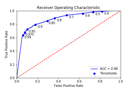
I ended up using a prediction threshold of 0.95, which means that if the query returned over 95% of the time there was an open spot at a block I would classify the block as having an open spot, and otherwise would classify it as being fully occupied. One of the reasons this threshold is so high is to minimize false positives, which in this case are predictions of a block having an opening that is actually fully occupied. From a user perspective, I would much rather say that a block is occupied and be wrong than say that a block is unoccupied and be wrong. It’s okay if a user passes by a block that was predicted to be full and it has an open spot. If the app directs a user to a block that is fully occupied, they are left to drive around and find a spot on their own, most likely cursing the app the entire time.

Building The Web App

Framework

Now that I had a way to make predictions about the availability of parking spots, I needed a way to make these easily accessible to an end user. I decided to use the Flask framework to build out a web-app. Flask is a Python framework, so I knew it would interact well with the code I had created already, and it would also allow me to integrate a web based front end to interact with the code. The official tutorial in the Flask documentation proved to be very useful in learning about the structure of a Flask project as well as how the front end web code could interact with the back-end Python code.

Back-End

I started with the back-end and built out several functions. I knew that I would want to take an address and a timestamp from the user on the front end and then be able to give them relevant predictions. To do this I built functionality to first geocode an address to a lat/long, then find blocks that were within a given radius to the point of interest, make predictions on the availability of these blocks, and finally package up the results in a GeoJSON format so that it could be plotted on a map on the front end.

Refactoring

The original back-end functions were quite long which made them difficult to read and to debug. In order to get them into a more manageable state, I started to refactor several of the functions. The goal of my refactoring was to maintain the original functionality of the code, but break it into a group of functions that each performed a singular task. With this goal in mind, I targeted functions that seemed to have multiple tasks in them and tried to find points where there was a single hand-off between sections of code. Once I had these sections of code identified, I was able to write a new function that completed the same steps and then call that new function inside the old function.

Testing

During this refactoring phase, I wanted to make sure that I was getting the same results from my functions given the same inputs. I ended up spending a good deal of time executing test cases almost line by line, and I figured there must be a better way. My mentor, Brian, introduced me to the pytest framework which was a formal and automated way to do the testing I was doing on my own. With a testing framework in place, I would be able to refactor some of my code and quickly test to make sure that I was getting the same results. I started by reading through some of the examples in the pytest documentation and then started to write some of my own tests. I initially wrote tests around the functions that I knew I was going to try to refactor. For instance I built a test to make sure that a given set of blocks was returned for a given set of coordinates from a function called findCloseBlocks(). I could then focus on refactoring the code while being able to quickly test the output to ensure I was getting the same results. Once I had completed the refactor of an individual function, I made sure to create tests for the new functions which I had introduced in the process. After going through a few iterations, my code was more readable and much easier to debug. The testing framework I put in place would also allow me to quickly ensure my code is still functioning if I ever wanted to make more changes. The new refactored code should allow the app to be more flexible and applicable to other potential use-cases.

Documentation

Another way to allow my code to be more extendable is to make sure that it is well-documented. I had plenty of comments in place throughout the code but had not implemented any formal docstrings along with the functions. I was introduced to Sphinx, which is a Python documentation generator. I went back though my code and documented each function in the Sphinx docstring format. Once that was complete, I was able to use Sphinx to automatically generate a directory of documentation for my code. Once I had my code hosted on GitHub, I was also able to use Sphinx to generate and host my documentation on ReadTheDocs.

Front-End

Once I had the back-end complete, I built out the user interface with a couple input forms and an interactive map using Leaflet. Leaflet is an open source JavaScript library for creating interactive maps on the web. The library allows the web app to pull map tiles from Open Street Map and also plot the relevant parking spaces for the user. It allows the user to be able to move the map around, click on different parking spots, and be able to interact with all of the information being presented. I didn’t have much experience with front end web code before this project and had a lot to learn about allowing for these types of interactions. I found the tutorials from MIT’s Department of Urban Studies & Planning to be very valuable in learning how to get the mapping portion of the project working as I intended. After working through some of the tutorials and linking up the front end interactions with the back-end functions I was able to serve up my predictions in an easily digestible format for the user.

Conclusion

This project started out with a conversation around how difficult it was to park in my new neighborhood. It became a full-stack data driven web app which can help users alleviate the pain of finding parking. The process started off with a search for a robust enough data set to perform some predictive modeling with. Once I had the a data set in hand and loaded into a database, I needed to spend time exploring the data. This started with making sure I understood the structure of the data and then diving into the values themselves. In this process I was able to gain some insights into the important features that have an effect on parking availability. With these insights, I started to build a model to predict the availability of parking in the future. This involved some initial parameter tuning to try to reduce error and some final threshold tuning at the end to focus on correctly predicting open parking spaces and reducing false positives. With the model in place, I then built out the web framework around it to allow for a user to easily interact with it. This included building out a Python based back-end and an HTML and JavaScript front end. This part of the project included some more traditional software engineering tasks like refactoring code, writing tests, and compiling documentation. At the end of it all, I have a piece of software that can accurately direct users to open parking spots.

Learnings

The breadth of this project allowed me to gain a deeper understanding of topics that I initially had a loose grasp on as well as experiment with and gain familiarity with a host of new tools that I hadn’t needed to use before:

• Agile Workflow – building out epics and sprints using JIRA
• MongoDB – NoSQL database technology and how to efficiently query it
• Exploratory Analysis – understanding data structure and features especially of a large data-set held in a database
• Model Building – extracting features from the data, training models and selecting error metrics, evaluating performance
• git – code versioning, and feature branching with pull requests
• Flask – building out back-end Python functions to interact with the frontend
• Javascript and HTML – creating a web page to allow for user interaction and to display model results
• Code Refactoring – increasing code readability and ability to manage with more modular code base
• pytest – creating test coverage allowing for efficient code refactoring and a more robust code base
• Sphinx – auto-generating documentation and creating complete and properly formatted docstrings
• AWS – launching an EC2 instance to run the app and deploy the model to the web

This project represents a big jump from simple projects that I had traditionally built out in Jupyter Notebooks, to a more production ready piece of software. I’m looking forward to building on this base going forward. I’m also hoping to petition the City of Boston to install parking sensors so I can use this app for myself!